Working for manufacturer engineering couple years. Sharing the manufacturing experience, skill, DFx, design, and information. Be care of this blog is personal share and content may not be 100% correctly.
Workingbear has already spent a good amount of time explaining what Cp (Precision) and Ck (Accuracy, sometimes called Ca) mean, and what each represents. We’ve also learned that using Cp or Ck alone can give an incomplete picture when it comes to quality control. So now, Workingbear is going to introduce the combined process capability index — Cpk — which is widely used today as a standard measure in statistical process control (SPC).
What Is Cpk in Process Capability?
Cpk is a comprehensive process capability index that takes both precision (Cp) and accuracy (Ck) into account. It provides a more realistic evaluation of how well a process performs.
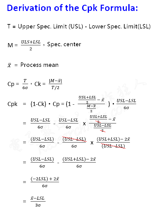
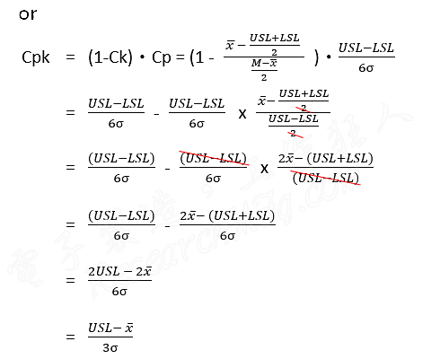
The formula for Cpk is: Cpk = (1 – Ck) × Cp
Basically, Cpk starts with Cp, then adjusts it by multiplying with (1 – Ck). This adjustment helps correct the potential blind spots of using Cp alone. The maximum value of (1 – Ck) is 1 — this occurs when Ck = 0, meaning the process average exactly matches the center of the specification. The further the process center shifts away from the spec center, the larger the Ck value becomes, and the smaller (1 – Ck) gets — which makes Cpk smaller too. A smaller Cpk means the process capability is worse.
Here’s a recap of the formulas:
Cp = T / (6σ) Where T = USL – LSL (Upper Spec Limit – Lower Spec Limit)
Ck = |M – X| / (T / 2) Where M is the spec center, X is the process mean (Use the absolute value because Ck is always a positive number)
Alternate Cpk Formula
There’s also another commonly used formula for Cpk: Cpk = min{(USL – X) / 3σ, (X – LSL) / 3σ}
This version takes the smaller value between the upper and lower side of the process distribution relative to the specification limits.
How to Calculate Cpk for One-Sided Specifications (Tolerances)
For a one-sided upper specification (tolerance), the Cpk is calculated as: Cpk = (USL – X) / 3σ
For a one-sided lower specification (tolerance), the Cpk is calculated as: Cpk = (X – LSL) / 3σ
Cpk Capability Level Assessment
Grade
Cpk Range
Interpretation
A
Cpk
≧
2.00
This process capability is very high, there’s no need for special inspections. You can easily achieve ppm-level quality (parts per million). When Cpk = 2.0, the defect rate is only 0.0020 ppm.
B
2.00
>
Cpk
≧
1.33
When the process capability is good, no inspection is required. Just maintain the current conditions. When Cpk = 1.66, the defect rate is about 0.6358 ppm.
C
1.33
>
Cpk
≧
1.00
This process capability is average, you can maintain the current state for about two months, but you should start looking for improvement actions. During this period, sampling inspections are necessary to monitor for any negative trends. When Cpk = 1, the defect rate is about 2700 ppm. When Cpk = 1.33, the defect rate drops to 66.08 ppm.
D
1.00
>
Cpk
This process capability is insufficient, immediate improvements must be made, and 100% inspection should be performed during this time.
Here are three distribution curves labeled A, B, and C, with the following explanations:
Curve A represents the best process capability. The process center aligns exactly with the specification center, and the distribution is narrow. You only need to keep monitoring—no adjustments are necessary.
Curve B also has the process center aligned with the spec center, but its distribution is wider and almost touches the upper and lower limits. This situation requires close monitoring or improvements.
Curve C has its process center shifted from the spec center, but the distribution is narrower than Curve B. In this case, simply adjusting the process to move the center closer to the spec center should solve the issue.


")

")


Leave a Reply